There are special filters in SecureSheet that are used to set up security for and filtering in a view.  These are set up in the Advanced Filter section and may be accessed when you edit a view.


Special Filters in SecureSheet

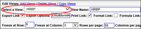
  1. Select the SecureSheet from your home page.
  2. Click Views. This puts you into View design in the Edit mode.

  1. Select the view you want to work with from the Select a View: drop-down.

  1. Modify the advanced filters as needed.


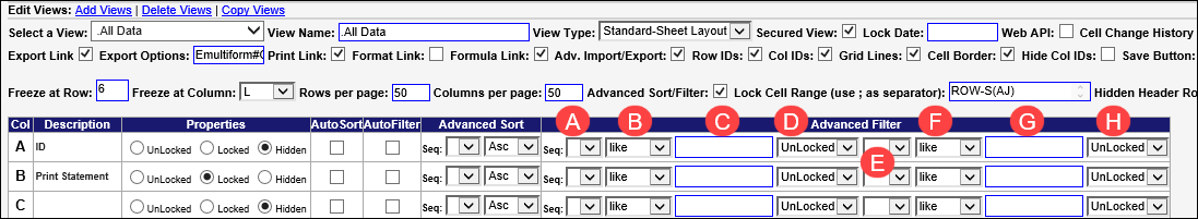
A.        Assign a Seq: to the advanced filter.  Up to three (3) columns can have advanced filters in a view.

B.        Select the condition to be used for the comparison , e.g., like, equals (=), not equal to (<>), less than (<), greater than (>), less than or equal to (<=), greater than or equal to (>=), In, Not In, not like. 

      • If you have a list, IN or NOT IN. In will return an exact match of your comparison text only. This logic says something is in the list.
      • If you have a partial string, LIKE or NOT LIKE. Like or not like assumes a wildcard prefix and suffix are assigned to the comparison text you enter. This logic looks for an exact match of the string found in the filter.
        • Like searches for a match inside the entire string, whereas In searches for a match on values separated by commas.
      • Use Not In to exclude value(s) from a column.
      • If you have a value as your comparison text, use a numeric operator (=, <=, >=, <>).

C.        Comparison text is the value that you want to compare the column to. In addition to normal values such as characters, numbers and dates, there are several special SecureSheet comparison filters that may be used. They are always bracketed by the number sign (#).

D.        UnLocked/Locked will lock or unlock the cells in this row if it is displayed by this filter comparison. This allows some rows to be displayed and the cells in the row unlocked for the user, while other rows may be displayed but all the cells locked for the user.

E.        Connector is used if you are applying more than one filter for the column. Select and/or to use with the next set of criteria.

F.        See Step 4B.

G.        See Step 4C.

H.        See Step 4D. 


SecureSheet Comparison Filter

Description

#email# 

Displays only those rows where the column contains the email address that matches the current login email address (as well as any blank rows). This is useful when you are trying to restrict the rows to a given user by their email address.

#now# 

Applies the condition for the comparison against the current date/time. For example, "show me all rows where Column C is less than now".

#today# 

Similar to #now#, except the comparison ignores time. Applies the condition for the comparison against the current date. For example, "show me all rows where column C is less  than today's date (no time)".

#?#

This is a "dynamic filter" that will dynamically prompt the user for the filter values in the view. This allows the values of the filters to be chosen at run-time by the user.

#list# 

Similar to #?# with the addition of a drop down list. This will dynamically prompt the user with a drop-down list to allow the user to select from existing values in the sheet for that specific column. This allows the value of the filters to be chosen at run- time by the user

    • When you use dynamic filters (#?# or #list#) in the comparison text field, the system will prompt the user for the filters at run time and use the label row (i.e., column header) to go get the descriptive text for the prompt (e.g.,  “Where Hire Date > ???”).
    • When you select dynamic filters (#?# or #list#) in the comparison text field, the system will prompt the user for the filters at run time and then display the rows that meet that criteria. 
    • Normally, after the query is run, the filter panel will close and the user will have to select a “Change Filters” link to re-open the panel. To keep filters open after a query is run, turn on the Keep filters open setting.

#cell, cell address# 

Applies the condition for the comparison against the cell value referenced. The cell address is used to find the value on the sheet that will be used in the filter. As an example, #cell,A5# would use the value in cell A5 for comparison in the filter.

#emailxref,name,email column,xref value column#

A comparison used to filter the rows of this sheet to the values in another sheet that are cross-referenced by email address. The email address of the person logged in will be used to find those filter values in the cross-referenced sheet. For example, a user may only be authorized to certain department codes and you only want to show rows to that user that have those department codes.

  • For example:  #emailxref,14;Users,A,B#
    • Filter parameters are:
      • #emailxref - this is the filter name and should not be changed.
      • 14 - or the SecureSheetID being referenced (only needed when a separate SecureSheet is being reference, e.g., the Users tab in the Users-Views SecureSheet).
      • name - this is the name of the tab in the SecureSheet (or a separate SecureSheet) that contains the cross-reference between email addresses and the corresponding valid values that they are able to see. NOTE:   The sheet name will like be Users from your Users-Views SecureSheet, and you must enter the SecureSheet ID (which can be found in Organization Statistics) followed by a semi-colon, and then the tab name. 
      • email column - this is the Column ID (e.g., A, B, C …) in the cross reference sheet that contains the email address.
      • xref value column - this is the Column ID (e.g., A, B, C …) in the cross reference sheet that contains the value to compare to.  You can designate multiple values to the same email by entering multiple column numbers separated by a semi-colon (ex. "B;C;D").  Alternatively, in a security set-up column in your Users tab in your Users-Views SecureSheet, you can designate multiple values for a given email for a specific column by separating the value with 3 asterisks "***" in the same column.
    • Where:
      • 14 is the SecureSheetID of the Users-Views SecureSheet
      • Users is the name of the tab in the Users-Views SecureSheet being referenced
      • A is the column in the Users tab that contains the user's email address
      • B is the column in the Users tab that is being cross referenced to the main sheet (e.g., EEID to EEID where Column F - EEID in the main compensation sheet contains this cross reference filter in the Advanced Filters)

SCENARIO: When employee should not see themselves in a view

  • When you are filtering on a column that is not an EEID, like a Business Unit or a Department, and the user is not supposed to see themselves in the results, add a second filter to the view (first filter would be on Business Unit or Department) on the EEID column Seq: x Not In emailxref,2;Users,A,B. This will automatically exclude them from the list.

NOTE:  If they are not supposed to see colleagues, this will not solve for that scenario. You would need to use another filter to remove a department, for example, or add a helper column to your main data tab that lists exclusions and filter on that.

#emailsqlxref#

A comparison used to filter the rows of this sheet to two or more security conditions that are required. 

  • The specific security conditions need to be identified in a security column in the Users tab (in the Users-Views SecureSheet) with a similar syntax to these examples:
    • (O In ('Chicago','St. Louis','Detroit'))-cols-O
    • (O = 'Chicago' And S = 'FINANCE')-cols-O,S
    • (O In ('Chicago','St.Louis') And S = 'OPS')-O,S
    • (H = 'Active' AND P NOT IN ('Human','HR') AND CF <> 'A')-cols-H,P,CF
  • And on the view that needs this security, put an advanced filter on Column A (typically) with the following syntax:  #emailsqlxref,2;Users,A,M#
      • Users is the name of the tab in the Users-Views SecureSheet being referenced
      • A is the column in the Users tab that contains the user's email address
      • M is the column in the Users tab that contains the SQL with the security that needs to be applied

SQL can also be used to show a roll-up view of a user's organization. The columns containing the organization structure in your main sheet will be referenced in the SQL statement (e.g., Col-AY = Manager Level 1, Col-AZ = Manager Level 2, etc.) in a security column the Users tab.

  • The SQL needs to be identified in a security column in the Users tab (in the Users-Views SecureSheet) with similar syntax to this example:
    • ="(AY="'&E4&'" OR AZ="'&E4&'" OR BA="'&E4&'" OR BB="'&E4&'")-cols-AY,AZ,BA,BB"
      • which will find the user name and return rows where the user name is found in any of the hierarchy columns (e.g., AY through BB in this example)
  • And on the rollup view, add an advanced filter on Column A (typically) with the following syntax:  #emailsqlxref,2;Users,A,L#
      • Users is the name of the tab in the Users-Views SecureSheet being referenced
      • A is the column in the Users tab that contains the user's email address
      • L is the column in the Users tab that contains the SQL with the rollup formula

#emailruxref#

An automatic rollup of the organization based on a 1:1 relationship of Employee:Manager.  As long as a manager is also an employee in the main data sheet, applying an automatic rollup filter is possible.

  • Add a rollup view, and on the column with the first line manager, set up an advanced filter with the following syntax:  #emailruxref,2;Users,A,B,G#
      • Users is the name of the tab in the Users-Views SecureSheet being referenced
      • A is the column in the Users tab that contains the user's email address
      • B is the Manager ID column in the Users tab
      • G is the column in the main data sheet with the EEID

DISTINCT

DISTINCT_ROW

Command that can be used in Summary Calcs on a View to pull unique instances from a column and place them in cells in the header rows, that you can then use in other header calculations.

  • The command only has to be placed in one cell and will then list the unique values vertically (DISTINCT) or horizontally (DISTINCT_ROW) for every unique instance.
  • On the Summary Calcs: line on the applicable View, use syntax K3=DISTINCT_ROW(F5:F2000)
    • For example:  The budget allocation needs to be the sum of all budgets a budget owner is responsible for, e.g., a manager has multiple departments that roll up to their total budget.
    • Use DISTINCT_ROW to lookup the unique budget owners. Then, through a formula that references the unique value found, lookup the department budget. Then, sum each department budget that is a match to the budget owner in a Total Budget header calculation that is displayed in their view.
  • If you use DISTINCT, which will display vertically, and you only have 10 header rows but 20 unique instances, for example, only the first ten unique instances will be displayed. If you need to list each one, consider DISTINCT_ROW as an option.
  • The DISTINCT results may be displayed or hidden on a view depending on their desired use.


Additional Notes on Special Filters:

  • When a filter cross-references a column on the main sheet to the Users tab in the Users-Views SecureSheet, the format needs to be consistent between the columns.
    • If there are leading zeros in the column on the main sheet that you are filtering on, the column in the Users-Views sheet also needs leading zeros.